Selecting the proper waveform and scan pattern are core considerations for imaging applications to ensure that the laser scanner performs its target function at high levels of accuracy.
WILLIAM R. BENNER JR., SCANNERMAX
Many photonics systems and methods require projecting lasers over an area of interest so that the reflected light can be sensed and interpreted. Among the most prominent examples are in the realms of imaging and ranging. These include confocal microscopy, lidar, and optical coherence tomography.

Courtesy of istock.com/Dmytro Naumov.
Techniques such as these support a range of industrial and biomedical applications. For each, the use of laser scanners is imperative to achieve system functionality.
Depending on the application, different waveforms can be used with laser scanners. The selection of the proper waveform to drive the scanner is vital to achieving the widest scan angle and the best possible image quality.
Laser-scanning fundamentals
There are three ways to move a laser beam to scan a pattern over an area of interest. The beam can be diffracted, which is achieved using acousto-optic (AO) beam deflectors; it can be refracted, using electro-optical (EO) scanners, such as Pockels cells; and it can be reflected, usually off a mirror mounted on a motor. Each method scans a line in 1D. Two scanners can be coupled to complete a scan of a 2D area.
Although AO and EO devices reach
favorable scan speeds up to ~100 kHz, both mechanisms present drawbacks. Notably, the scan angles that the devices offer are only a few degrees or less; beam size is limited to a few millimeters; and, for AO devices specifically, they cannot scan multiple wavelengths simultaneously. AO devices also fail to deliver desirable levels of optical throughput.
Reflection scanning is performed by mechanical scanners rotating a physical mirror. This allows a wide scan angle that can exceed 90°, with beam diameters
of up to 50 mm. Optical throughput is typically very high, and multiple wavelengths can be deflected simultaneously.
However, because a physical mirror is being moved during these scans, mechanical scanning is slow relative to the AO and EO methods.
Galvanometer scanners
Three forms of scanning exist under the umbrella of mechanical scanning: polygon, resonant, and galvanometer. Polygon and resonant scanning use mirrors to scan the same area repeatedly, typically at fixed angular amplitude(s). In contrast, galvanometer scanning systems can position a beam anywhere within the scan area at any time — making them the most versatile type of mechanical scanner.
Galvanometer scanners are widely used in imaging applications due to their high flexibility. Commonly, end users deploy two galvanometers with mirrors on their shafts in combination. In such an architecture, the laser beam is reflected off one mirror, which is scanned horizontally onto a second mirror, which scans vertically. This combination allows the beam to be placed anywhere in a rectangular scan field and allows pairs of galvanometers to draw complex patterns. Supported applications span optical layout templates, or ply alignment, as well as laser projection of vector graphics.
In many cases, end users are unaware of the simple scanning patterns and optimizations that can be used to repetitively scan a beam over an area of interest. With source signals obtained from computer output, a user can easily maintain full control over the waveshape and the relative timing of the x and y signals.
Covering the area of interest
The most common scan pattern for systems and applications is a raster. This pattern features an x-axis scanner, which is responsible for scanning horizontal lines, and a y-axis scanner, which steps the lines vertically down the area of interest. The x-axis moves faster, sweeping the beam back and forth hundreds or even thousands of times per second. The y-axis moves the horizontal lines downward and may be operated in the range of 1 to 100 Hz, depending on the desired number of lines of horizontal sweep.
To generate a raster, the x-axis scanner can be fed with a sine wave, triangle wave, or sawtooth wave as well as by feeding the y-axis scanner with a stepped waveform that positions the y-axis on each next line.
Figure 1 shows a triangle wave driving the x-axis scanner, and a stepped sawtooth on the y-axis. The black lines represent a constant velocity triangle wave and the dashed blue semicircles moving at the edges represent the y-axis scanner stepping downward as the x-axis scanner turns around. The diagonal blue line represents the final retrace of the y-axis.
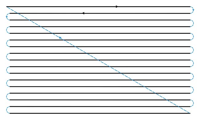
Figure 1. In this raster scanning system, a triangle wave is used on the x-axis with a stepped sawtooth on the y-axis. The dark lines represent a constant velocity triangle wave. The dashed blue lines at the edges represent the y-axis scanner stepping downward while the x-axis scanner turns around, amid the final retrace of the y-axis (dashed blue line). Courtesy of ScannerMAX via William Benner Jr.
In this sequence, all the lines remain completely horizontal since a stepped sawtooth is used on the y-axis. Whereas, if a regular sawtooth was used on the
y-axis, the beam direction would always be downward, even on the horizontally scanning lines. As a result, the lines would be diagonal using a conventional sawtooth (Figure 2).
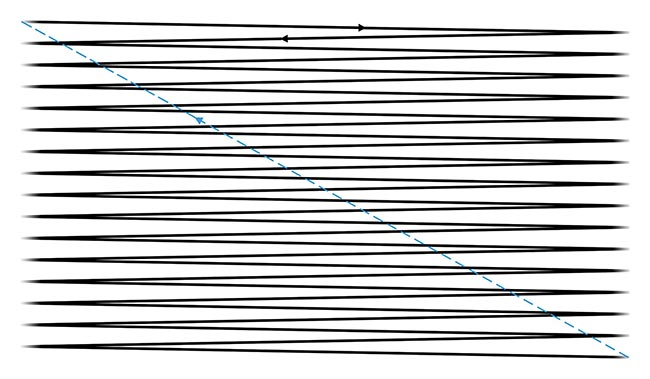
Figure 2. The scan sequence from Figure 1 with the use of a conventional sawtooth instead of a stepped sawtooth. The lines in the sequence are diagonal, with the beam direction constantly traveling downward. Courtesy of ScannerMAX via William Benner Jr.
Though a galvanometer is not the only option for such a system, an x-y galvanometer scanning system is very useful. For example, it can scan each waveform type and can jump from point to point and hold a position indefinitely if desired for the application. Moreover, galvanometers can change their scan extent to “zoom” into a particular area and can change the offset to “pan” around a prospective image.
Telling the scanner where to go
Galvanometer scanning systems accept an input referred to as the “command” input. The scanning waveforms sine, triangle, and sawtooth are fed to the command input of the servo system as a periodic series of samples.
In many cases, end users are unaware of the simple scanning patterns and optimizations that can be used to repetitively scan a beam over an area of interest.
The mirror angle that is achieved
during scanning is referred to as the
position. Since galvanometers are electro-mechanical systems, the mirror angle (position) cannot instantly achieve the angle requested by the command input. This causes a delay in time between
the command and the actual mirror position during operation. For the same reason, the mirror position is unable to completely track the incoming command signal through all amplitudes and frequencies, which are other highly important values influencing the scan system sequence.
Although this dynamic can be easily understood for galvanometer scanners, and indeed all laser scanners, the subject of laser scanning can present challenges. This is especially true for electrical engineers — who are most commonly tasked with integrating these scanners into a product. As a result, conceptual models tailored for these engineers aid greatly in their understanding and quick implementation.
Consider, for example, a properly tuned galvanometer scanning system — galvanometer scanner motor plus servo driver. This system behaves much like a low-pass filter used in electronics. The circuit in Figure 3 is a simplified model that shows the behavior of the scanning system and how the mirror position tracks the command signal, while also driving the galvanometer coil. The corresponding frequency response graph in Figure 4 shows how the amplitude of the position signal “rolls off” as frequency increases. The diagram specifically shows a –3-dB bandwidth of 2.5 kHz.
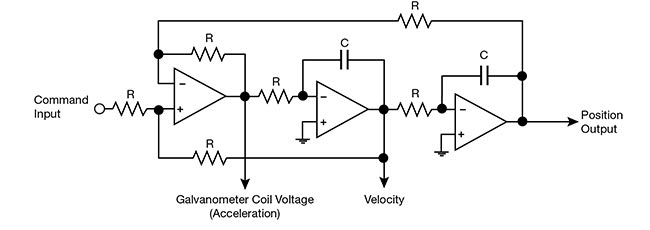
Figure 3. A two-pole low-pass filter model illustrating how the mirror position tracks the command signal, while driving coil voltage in a galvanometer scanning system. Courtesy of ScannerMAX via William Benner Jr.
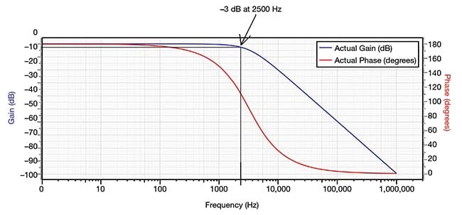
Figure 4. A –3-dB bandwidth of 2.5 kHz is shown as the amplitude of the position signal “rolls off” as frequency is increased. Due to the low-pass filter action, the higher the scan frequency, the greater the roll-off of the real position. Courtesy of ScannerMAX via William Benner Jr.
In Figure 3, a command input (waveform) is sent to the servo driver, which sends voltage to the coil so that the motor accelerates. This acceleration establishes velocity, which in turn affects the position of the motor and mirror.
Per this multistep sequence, the mirror’s actual position will always lag behind the command input. Insofar as it relates to low-pass filtering, low-pass filter action dictates that a higher scan frequency corresponds to a greater roll-off, or rounding, of the actual position.
Delay, step time, and position error
Detecting and understanding errors that may arise during the scan process is necessary to realize the simplicity that a properly functioning system delivers to an application. In Figure 5, for example, a triangle wave is fed to the command input (yellow) with the mirror position (pink). This oscilloscope image shows an obvious delay between command and position. It also shows that the position waveform does not quite achieve the same amplitude as the command. Further, the position has a rounded top and bottom, which is caused by the low-pass filter action of the servo/scanning system.
The delay between the command and position is called a tracking delay. As long as the operational amplifiers, as shown in Figure 3, do not saturate, this tracking delay will remain consistent regardless of the amplitude or slope of the command signal.
However, if the slope of the command input changes direction — which it does twice per cycle in a triangle wave — it will take the position some time to change direction and start traveling at the new slope rate. This amount of time is referred to as the step time or settling time.
This delay between command input and position also means that the command arrives to request a position before it is achieved. Therefore, if the command
is changing, this time delay causes a
difference in the angle between command and position. This difference in angle is referred to as position error (Figure 5).
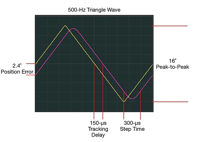
Figure 5. This oscilloscope screenshot shows a 500-Hz triangle wave fed to the command input (yellow), with the mirror position (pink) and the delay between command and position. Courtesy of ScannerMAX via William Benner Jr.
Constant velocity
For most imaging applications, it is desirable to maintain constant velocity during the entire length of each scan line. However, some portions of the waveform must be dedicated to slowing and reversing the scanning direction in preparation for the arrival of the next scan line or scan field. Scanning efficiency is the ratio of time spent in constant velocity to the total amount of time in one cycle.
Figure 6 shows a 600-Hz triangle wave, with servo gains set such that the tracking delay is 90 μs. The total scan angle is
14°, of which 11° are in constant velocity. This is the maximum scan angle possible for this frequency, with this servo tuning, and using a standard triangle-wave input since the coil voltage parameter is nearly touching +/−20 V.
A white trace shows the position during the times when the beam is traveling at constant velocity in Figure 6 (blue). For this scanning scenario, the velocity is constant at 16,800°/s for 78% of the time. However, there are short periods when
the mirror must slow down, turn around, and speed up again. These areas (pink) correspond with the step time of the
scanner, which is 180 μs for the servo tuning shown.
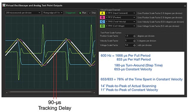
Figure 6. When the beam is traveling at constant velocity (blue), the position is highlighted (white). The velocity is constant, but there are short periods of time when the mirror must slow down, turn around, and speed up again. These areas (pink) are not highlighted and correspond with the scanner’s step time. Courtesy of ScannerMAX via William Benner Jr.
Because the beam must be turned off during the period when the scanner is turning around, less than the full 14° would be usable for an imaging application that requires constant velocity.
At 16,800°/s, the position error for this tuning is 0.75 mechanical degrees, or
1.5 optical degrees, which must be subtracted from both peaks of the triangle wave, giving a useful scan angle of 11 optical degrees peak-to-peak. With the traveling in constant velocity for 78% of the time, the overall scanning efficiency is 78%.
Avoiding saturation: cycloid approach
The scan angle in Figure 6 could not be increased because the coil voltage was already at the maximum recommended +/−20 V: As shown, the coil voltage peaks occur at the “tips” of the triangle wave, where the command input is changing the slope. Any increase in scan angle would result in exceeding this voltage limit, which would cause overshoots and distortion in the actual scanning.
However, it is possible to reduce the rate of change of the slope at the tips of the triangle wave, which would enable operation at a larger scan angle. This is performed by “rounding” the tips of the triangle wave. The optimal way to achieve this is to replace the tips of the triangle wave with half of a sine wave.
To replace the tips of the triangle wave with half of a sine wave — completed via the cycloid approach — the triangle wave is broken into two separate ramp portions. One ramp portion is ascending and one is descending. A small amount of time is allotted between each ramp portion for the half sine wave to be inserted. Also, the amplitude of the half sine wave is adjusted so that the position, velocity, and acceleration all match. This provides a smooth transition between the ramp and sine wave portion.
In Figure 7, Tramp represents the amount of time allotted for each ramp portion and Trs represents the amount of time allotted for each half sine wave. Letter A represents the amplitude of the ramp portion, with A0 and A1 representing the start and finish of the sequence, respectively. Alpha represents the amplitude of the sine wave portion.
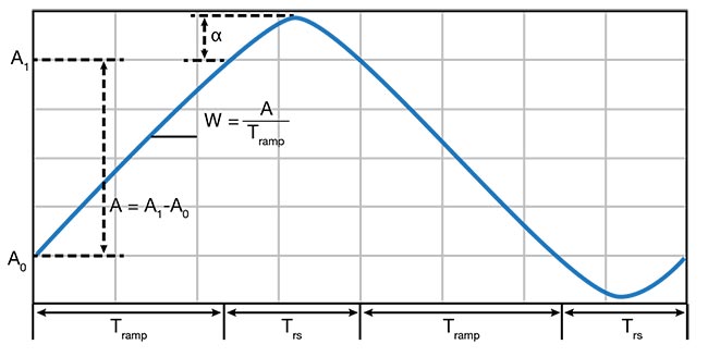
Figure 7. The cycloid approach replaces the tips of the triangle wave with half of a sine wave. Tramp represents the amount of time allotted for each ramp portion; Trs represents the amount of time allotted for each half sine wave. Letter A represents the amplitude of the ramp portion; A0 and A1 represent the start and finish, respectively. Alpha represents the amplitude of the sine wave portion. Courtesy of ScannerMAX via William Benner Jr.
Figure 8 shows this same principle, where the triangle wave can be compared with the cycloid wave. The derivative waveforms are also shown to indicate velocity, which is constant during the ramp portions and changing smoothly and symmetrically between the ramp portions.
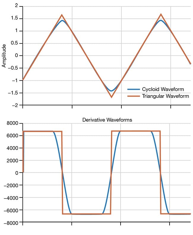
Figure 8. The triangle wave compared with the cycloid. The derivative waveforms are also shown, to indicate velocity. Courtesy of ScannerMAX via William Benner Jr.
Figure 9 incorporates a triangle wave modified using the cycloid approach shown in Figures 6 and 7. Specifically, half sine waves lasting 325 μs are inserted to enable an increase of the total scan angle to 36°, of which 22° is in constant velocity. The usefulness of cycloids for triangle-wave scanning is evident, since the coil voltage is no greater than in Figure 6, but the usable scan angle with constant velocity has doubled, with no additional change to oscilloscope scale factors in Figure 6.
Figure 9. A triangle wave modified using the cycloid approach shows the benefit of cycloids for triangle-wave scanning. Courtesy of ScannerMAX via William Benner Jr.
The velocity in the scanning scenario shown in Figure 8 is constant at 48,292°/s for 61% of the time (white portions of
the position trace). The time periods
dedicated to slowing the mirror and turning around are the pink portions of the position trace and correspond to the
180 μs step time of the scanner. An additional 325 μs is also added for the half sine waves that make up the cycloid
portion of the waveform.
At 48,292°/s, the position error for this tuning is 2.18 mechanical degrees, or
4.36 optical degrees, which must be subtracted from both peaks of the ramp portions of the triangle wave to accurately gauge the scan system performance and influencing values. The amplitude of each half sine wave is 2.62°, giving a useful scan angle of 22 optical degrees peak-to-peak. Since the beam is traveling at constant velocity for 61% of the time, the overall scanning efficiency is 61%.
Meet the author
William R. Benner Jr. is president and CTO of Pangolin Laser Systems and project leader for the ScannerMAX division. He holds more than 50 patents spanning actuators, position sensors, and lenses used for laser projection applications; email: [email protected].