Deciphering FLIM images remains a challenge, but a graphical representation of data collected from multiple images may unlock insights.
YUANSHENG SUN, SHIH-CHIU JEFF LIAO, AND BENIAMINO BARBIERI, Barbieri, ISS INC.
With the peculiar selectivity of probes, fluorescence lifetime imaging (FLIM) can provide quantitative information about the probe microenvironment, including the presence of ions, pH, oxygen, viscosity, and electrical signals. This capability has proved to be valuable in key life sciences research areas, such as in the detection of molecular/protein interactions, molecular environment sensing, drug development, and metabolic imaging for studying cancer as well as neurodegenerative, diabetes, cardiovascular, and respiratory diseases. Traditional methods for determining fluorescence decay times involve fitting analysis at each image pixel, which requires expertise in selecting fitting models and statistical tools. It is time-consuming and hampers FLIM applications. In response, a graphical method, called the phasor plots, has been developed, bypassing assumptions about specific decay modeling1.
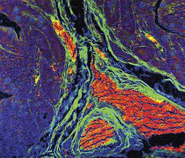
A merged image showing false hematoxylin and eosin stains, created with the multi-image phasor analysis (MiPA) approach to fluorescence lifetime imaging (FLIM). Courtesy of ISS Inc.
This article will highlight the potent techniques of phasor plots-based quantitative FLIM analysis, leveraging the multi-image phasor analysis (MiPA) approach. Various applications will be outlined, including time-resolved multiplexing, label-free nicotinamide adenine dinucleotide (NADH) imaging, stimulated emission depletion (STED) superresolution imaging, and Förster resonance energy transfer (FRET) imaging.
The phasor plot
The phasor plot is a graphical representation of raw FLIM data (Figure 1). Each pixel in a FLIM image is transformed to a point on the phasor plot. Its coordinate is defined by the G (x-axis) and S (y-axis) values (Figure 1a) in the following mathematical equation: g = m × Cos (φ) and s = m × Sin (φ), where m and φ are the modulation ratio and the phase delay measured at a particular modulation frequency in the frequency domain (Figure 1b). The phasor transformation can be applied to the time-domain decay data, such as time-correlated single photon counting through the Fourier transform (Figure 1c,d). The phasor plot is drawn from raw FLIM data. The relationship between phasor and lifetime is given by:
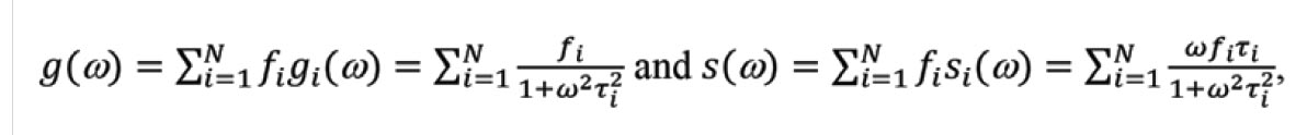
where N is the number of lifetime species, and fi is the contribution of the ith lifetime species (τi) to the total intensity. ω (= k × 2πF, k = 1, 2, 3 …) is called the angular modulation frequency and can be a kth-order harmonic of the repetition frequency (F) of the pulsed excitation source. For single-exponential species, the phasor coordinate resides on a semicircle centering at (g = 0.5, s = 0) with a radius of 0.5, commonly referred to as the universal semicircle.
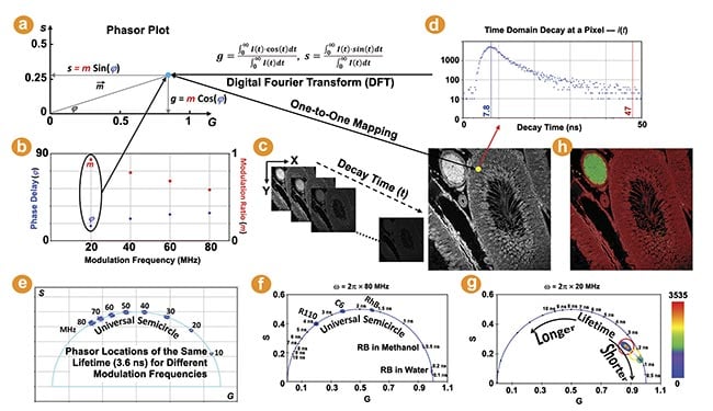
Figure 1. The phasor plot illustration. Each pixel in a fluorescence lifetime imaging (FLIM) image is transformed to a point on the phasor plot (a). m and φ are the modulation ratio and phase delay measured in the frequency domain (b). The phasor transformation can be applied to the time domain decay data using the Fourier transform (c,d). The lifetime shifts counterclockwise with increasing modulation frequencies. The phasor plots of five FLIM images of fluorescent dyes in solution (f). The raw FLIM image shown (c) is plotted on the phasor plot (g). The pixels belonging to the phasor population selected by each cursor are highlighted (h). Courtesy of ISS Inc.
The universal semicircle is an explicit ruler for the lifetime values of single-exponential species. Its scale, however, depends upon the angular modulation frequency (ω) used for drawing the phasor plot. For time-correlated single photon counting and digital frequency domain FLIM, wherein phase and modulation are measured simultaneously, phasor plots can be drawn using the laser repetition frequency or its higher harmonic frequencies. A higher frequency increases the “s/g” ratio for the same lifetime, resulting in its phasor coordinate shifting counterclockwise along the semicircle (Figure 1e). The phasor plots of two frequencies (20 MHz and 80 MHz) are compared, showing that the lifetimes within 3 ns are more spread out in the 80-MHz plot (Figure 1f) while the lifetimes between 5 and 10 ns are better separated by using 20 MHz (Figure 1g). This demonstrates a wide flexibility in selecting a proper modulation frequency for the phasor plot to visualize and contrast different lifetimes.
The value of a single-exponential lifetime can be directly obtained from its phasor coordinate on the semicircle. Figure 1f shows the phasor plots of the raw FLIM images of several fluorescent dyes in solution acquired by FastFLIM at room temperature. As expected, the phasor distributions of these single-exponential species fall on the semicircle and their lifetimes are directly resolved by their phasor coordinates on the semicircle.
The phasor coordinate of a multiexponential species, which would likely be statistically representative of a biological specimen, falls inside the semicircle. While the lifetime value of a complex species is not directly derivable from its phasor coordinate, its change can be easily identified on the phasor plot: Following the semicircle ruler, lifetimes decrease clockwise toward (1,0) as the zero lifetime and increase counterclockwise toward (0,0) as the infinite lifetime. Figure 1g shows the phasor plot of the raw FLIM image given by Figure 1c. The entire phasor distribution falls inside the semicircle, indicating that all the pixels have multiexponential species. The density, or number, of pixels that fall on the same phasor coordinate is indicated by a colored heat map.
Every image pixel is mapped to a specific coordinate on the phasor plot representing lifetime information. This mapping enables the easy identification of the pixels in images (not limited to one in MiPA) corresponding to a phasor distribution of the same lifetime signature. Vice versa, the phasor plot can be drawn using only the pixels selected within regions of interest to visualize and analyze their phasor distributions. In MiPA, available in the ISS VistaVision software, users can activate various cursors of different colors and shapes, such as circle, oval, square, and rectangle, with adjustable sizes to select populations of distinct lifetime signatures shown by the phasor plots. For example, in the phasor plot (Figure 1g) of the image shown in Figure 1c, three colored cursors are used to select the major phasor populations with the longer lifetime (red) and the minor phasor populations with the shorter lifetime (green) as well as the points between them (yellow); the pixels in the image belonging to the phasor population selected by each cursor are highlighted by its color at 50% transparency (Figure 1h).
Time-resolved unmixing by MiPA
Using time-resolved photon information with phasor plot-based unmixing enhances image quality and quantification, making it particularly valuable for biological research that requires precise measurements, such as in the study of protein-protein interactions and cellular signaling. In addition, lifetime, akin to spectra, is an inherent fluorophore property distinguishing it from others. Thus, the FLIM-phasor unmixing enables multiplexing by using fluorescent dyes of the same color but different lifetimes.
The phasor coordinate of a two-species mixture aligns with the line connecting the phasor coordinates of each individual species. The MiPA two-species unmixing process is illustrated by Figure 2a. It calculates the fraction of each species per pixel, resulting in two separate images comprising only photons emitted by each species. Figure 2b depicts the two-species unmixing of a sample containing both Rhodamine B and Rhodamine 110 dyes in water. Figure 2c-e show the multiplexing capability by using MiPA two-species unmixing to quantitatively separate two fluorescent species of different lifetimes in a Convallaria (flowering plant) sample.
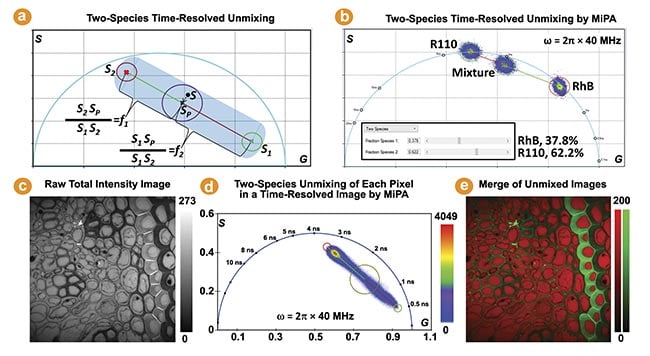
Figure 2. The two-species time-resolved unmixing by multi-image phasor analysis (MiPA). Two cursors are used to mark the phasor coordinates of the two individual species (S1, S2) to resolve a mixture species of them (Sp) (a). This is applied to a mixture of dyes in water using the phasor plots of the fluorescence lifetime imaging (FLIM) images acquired from the mixture and both individual species (b). The FLIM image’s phasor plots from a Convallaria sample reveal a linear distribution, suggesting the contributions of two distinct lifetime species at each pixel. Shorter and longer lifetime species are marked by green and red cursors, respectively (c-e). Courtesy of ISS Inc.
The phasor coordinate of a three-species mixture lies in a triangle bounded by the phasor coordinates of the three individual species. The MiPA three-species unmixing process is illustrated by Figure 3a. It calculates the fraction of each species for every pixel, producing three separate images containing only the photons emitted by each species. Figure 3b shows the phasor plots of three fluorescent dyes (rose bengal, Rhodamine B, and Rhodamine 110) in water and their mixtures.
The MiPA three-species unmixing explicitly resolves the contribution of each species to the total intensity of the mixture, which is useful for studying complex properties and dynamics of cells and tissues. This method is employed on a FLIM image obtained from a hematoxylin and eosin-stained tissue sample to quantitatively separate three lifetime species, enabling visualization of their distribution and overlap within the tissue (Figure 3c-e). It is noteworthy the phase plot-based unmixing can separate more than three species, by leveraging the phasor plots generated from multiple modulation frequencies2.
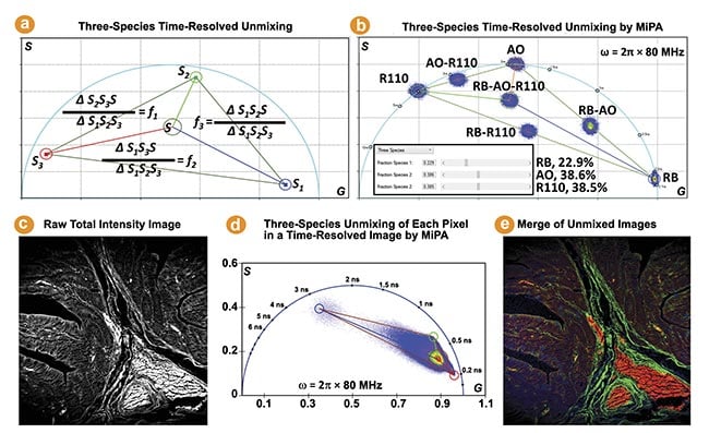
Figure 3. The three-species time-resolved unmixing by multi-image phasor analysis (MiPA). Three cursors are used to mark the phasor coordinates of the three individual species (S1, S2, S3) to resolve a mixture species of them (Sp) (a). The phasor plots of seven fluorescence lifetime imaging (FLIM) images (b). The phasor plot of the FLIM image acquired from a hematoxylin and eosin-stained tissue sample reveals a triangle distribution, suggesting the presence of three distinct lifetime species. The shortest, intermediate, and longest lifetime species are identified by positioning red, green, and blue cursors at the three extreme corners of the distribution (c-e).
Courtesy of ISS Inc.
Label-free NADH FLIM by MiPA
For analyzing a biexponential species, MiPA calculates the fractions of the two lifetime components as well as the intensity and amplitude weighted lifetimes (Figure 4a). Figure 4b shows the two-component analysis of a sample containing both Acridine Orange and Rhodamine 110 dyes in water. Analyzing cellular NADH FLIM data usually involves fitting biexponential decays to distinguish between free, or fast component, and bound, or slow component, forms. This complexity is simplified by MiPA (Figure 4c,d). Given the free NADH’s phasor coordinate obtained from measuring the free NADH solution, MiPA derives the lifetime for the bound form of the cellular NADH. MiPA offers various denoising filters, such as mean, median, Gaussian, and their combinations, and intensity thresholding for robust results (Figure 4e) and creates cellular NADH maps for free and bound fractions, free-to-bound ratios, and average lifetimes (Figure 4f-h). It offers an effective and robust method of tracking dynamic changes in metabolic states within live cells, tissues, and organisms.
![Figure 4. The two-component analysis by multi-image phasor analysis (MiPA) for label-free nicotinamide adenine dinucleotide (NADH) fluorescence lifetime imaging (FLIM). Two cursors are used to mark the phasor coordinates of the two single-lifetime components to resolve a biexponential species of the two components (a). Using three FLIM images, MiPA calculates the mixture’s intensity-weighted (t1 f1 + t2 f2) and amplitude-weighted (t1 t2/[t2 f1 + t1 f2]) average lifetimes (b). MiPA derives the lifetime of the cellular NADH-bound form (c-e). MiPA produces cellular NADH maps depicting the free and bound fractions, the free-to-bound ratios, and average lifetimes (f-h). Courtesy of ISS Inc.](/images/Web/Articles/2024/4/30/Feat_FLIM_Fig4.jpg)
Figure 4. The two-component analysis by multi-image phasor analysis (MiPA) for label-free nicotinamide adenine dinucleotide (NADH) fluorescence lifetime imaging (FLIM). Two cursors are used to mark the phasor coordinates of the two single-lifetime components to resolve a biexponential species of the two components (a). Using three FLIM images, MiPA calculates the mixture’s intensity-weighted (τ1 f1 + τ2 f2) and amplitude-weighted (τ1 τ2/[τ2 f1 + τ1 f2]) average lifetimes (b). MiPA derives the lifetime of the cellular NADH-bound form (c-e). MiPA produces cellular NADH maps depicting the free and bound fractions, the free-to-bound ratios, and average lifetimes (f-h).
Courtesy of ISS Inc.
SPLIT-STED by MiPA
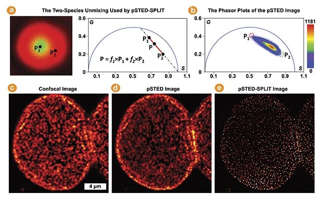
Figure 5. The pulsed stimulated emission depletion (pSTED)-separation by lifetime tuning (SPLIT) by phasor plots in multi-image phasor analysis (MiPA) for enhancing STED resolution. The phasor of each pixel in a pSTED fluorescence lifetime imaging (FLIM) image is a linear combination of two-lifetime species denoted by P1 (in the doughnut center, wanted) and P2 (in the doughnut crest, unwanted) (a). Using a pSTED-FLIM image and applying the two-species unmixing, the SPLIT technique accurately segregates the desired photons emitted from the doughnut center from the unwanted photons (b). Confocal, pSTED, and pSTED-SPLIT images of a nuclear pore complex labeled with Star635 dyes in Cos7 cells (c-e). Courtesy of ISS Inc.
The time-resolved pulsed STED (pSTED) image encodes information about distinct decay kinetics, reflecting the fact that molecules may interact with either the excitation beam alone or both the excitation and depletion beams (Figure 5a). The separation by lifetime tuning (SPLIT) technique employs phasor plot analysis to decode various decay kinetics, effectively segregating desired photons with specific decay characteristics (i.e., excitation solely at the doughnut center) from those emitted by incompletely depleted molecules (Figure 5b).
This enhances spatial resolution without intensifying the depletion beam or introducing artifacts, as demonstrated by comparing the confocal, pSTED, and pSTED-SPLIT images of a nuclear pore complex labeled with Star635 dyes in Cos7 cells (Figure 5c-e)3. Insights derived from better-resolved nuclear structural information in intact cells have been invaluable to studies of genetics and replication.
FRET trajectory analysis by MiPA
FLIM provides one of the most robust methods for measuring FRET in live specimens4. Changes in FRET can be easily identified from the phasor plots of raw FLIM data. The FRET calculator in MiPA, developed based on the FRET trajectory method and illustrated in Figure 6a, can accurately determine the FRET efficiency (E) per pixel, enabling quantification and localization of FRET within biological samples5. This is an effective way to track protein-protein interactions in live cells. Figure 6b,c shows an example of MiPA being used to visualize and quantify changes in FRET in live cells expressing the Cerulean-5aa-Venus (C5V) construct during acceptor bleaching. The Cerulean (donor) and Venus (acceptor) fluorescent proteins are tethered by a 5 amino acid linker.
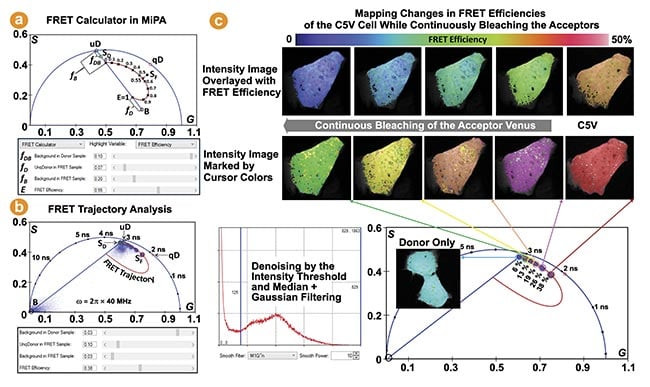
Figure 6. The Förster resonance energy transfer (FRET) trajectory analysis in multi-image phasor analysis (MiPA) for fluorescence lifetime imaging (FLIM)-FRET. The phasor measured from a FRET sample (SF) is decomposed into three species: the background (B), whose phasor coordinate can be given from background pixels or measuring unlabeled samples; the unquenched donor (uD), whose phasor coordinate is obtained from measuring the donor-only control sample (SD) and considering its background contribution (fDB); the quenched donor (qD), whose phasor coordinate is for a particular FRET efficiency (E) is determined given the unquenched donor phasor coordinate and the relationship “τDA = τD × (1-E)” (a). The FRET trajectory curve is drawn for the phasor plots of the FLIM images, measuring the donor (Cerulean) in live cells expressing the Cerulean-5aa-Venus (C5V) FRET standard construct, while continuously bleaching the acceptor (Venus) (b). The C5V phasor plots reveal increased dequenching (lifetimes) of the donor following more bleaching of the acceptor, illustrated by their counterclockwise movement along the semicircle (c). Courtesy of ISS Inc.
FLIM analysis in the future
The challenge of FLIM data analysis in life sciences lies in achieving both robustness and speed, given the limited photon counts per pixel and large data sets, which are typically hundreds of times larger than steady-state intensity images. Phasor plots offer a potential solution to this dilemma. Only two parameters (g,s) per pixel are required by the phasor plot analysis, significantly reducing data complexity compared to fitting a decay histogram with hundreds of time bins to account for multiple data points per pixel.
In addition, from raw FLIM images, pixels with the same lifetime signature falling at the same phasor coordinate are binned together for the analysis, making it a robust global analysis to deal with insufficient photon counts per pixel. This is a common problem for analyzing complex decay dynamics in FLIM; yet this binning process by the phasor plots is completely unbiased compared to the spatial binning typically used by fitting. The user-friendly interface and quantitative capabilities of MiPA can empower researchers to fully leverage the benefits of phasor plots, enabling them to tackle more intricate challenges.
Meet the authors
Yuansheng Sun received his Ph.D. in biomedical engineering from the University of Iowa and was further trained in the Keck Center for Cellular Imaging at the University of Virginia. He is now working at ISS Inc. as director of microscopy and spectroscopy; email: [email protected].
Shih-Chu Jeff Liao received his Ph.D. in biomedical engineering from Case Western Reserve University. He has more than 25 years of experience as a research scientist in microscopy at ISS Inc.; email: [email protected].
Beniamino Barbieri graduated with a degree in physics from the University of Pisa, Italy, where he worked on high-resolution laser spectroscopy. He joined ISS in 1986 and has been president of the company since 1992; email: [email protected].
References
1. S. Ranjit et al. (2018). Fit-free analysis of fluorescence lifetime imaging data using the phasor approach. Nat Protoc, Vol. 13, No. 9, pp. 1979-2004.
2. A. Vallmitjana et al. (2020). Resolution of 4 components in the same pixel in FLIM images using the phasor approach. Methods Appl Fluoresc, Vol. 8, No. 3, p. 035001.
3. G. Tortarolo et al. (2019). Photon-separation to enhance the spatial resolution in pulsed STED microscopy. Nanoscale, Vol. 11, No. 4, pp. 1754-1761.
4. Y. Sun et al. (2011). Investigating protein-protein interactions in living cells using fluorescence lifetime imaging microscopy. Nat Protoc, Vol. 6, No. 9, pp. 1324-1340.
5. M.A. Digman et al. (2008). The phasor approach to fluorescence lifetime imaging analysis. Biophys J, Vol. 94, No. 2, pp. L14-L16.